第 5 章:高斯消元法
本章介绍高斯消元法,这是一种求解线性方程组的方法。这类方程组在处理实际问题中经常遇到,例如这个计算机视觉问题:给定物体的若干张图像,计算物体的三维模型。 图 5.1 展示了 Örebro 城堡的四张图像。利用这些图像以及另外 667 张类似图像,可以计算出图 5.2 所示的点云。这些计算包括求解许多方程组。高斯消元法是学习这类方程组的很好途径。有关此例子的更多信息,请参阅此YouTube 视频。

熟悉方程组的一种方法是考察两条直线相交时会发生什么。
要在平面中描述一条直线,许多人首先遇到的记法之一是
| \begin{equation} y = kx + m, \end{equation} | (5.1) |
| \begin{equation} ax + by + c = 0 \end{equation} | (5.2) |
| \begin{equation} \begin{cases} 2 x + 3 y = -5,\\ 5 x + 2 y = 4. \end{cases} \end{equation} | (5.3) |
交互图 5.4 展示了当两条直线方程改变时,两条直线的交点,即诸如 (5.3) 这类方程组的解,如何交互式地变化。
本章介绍一种称为高斯消元法的系统方法,用于分析和求解这类方程组。不过, 我们首先再从几个线性方程的例子开始。
例 5.1:
视频压缩
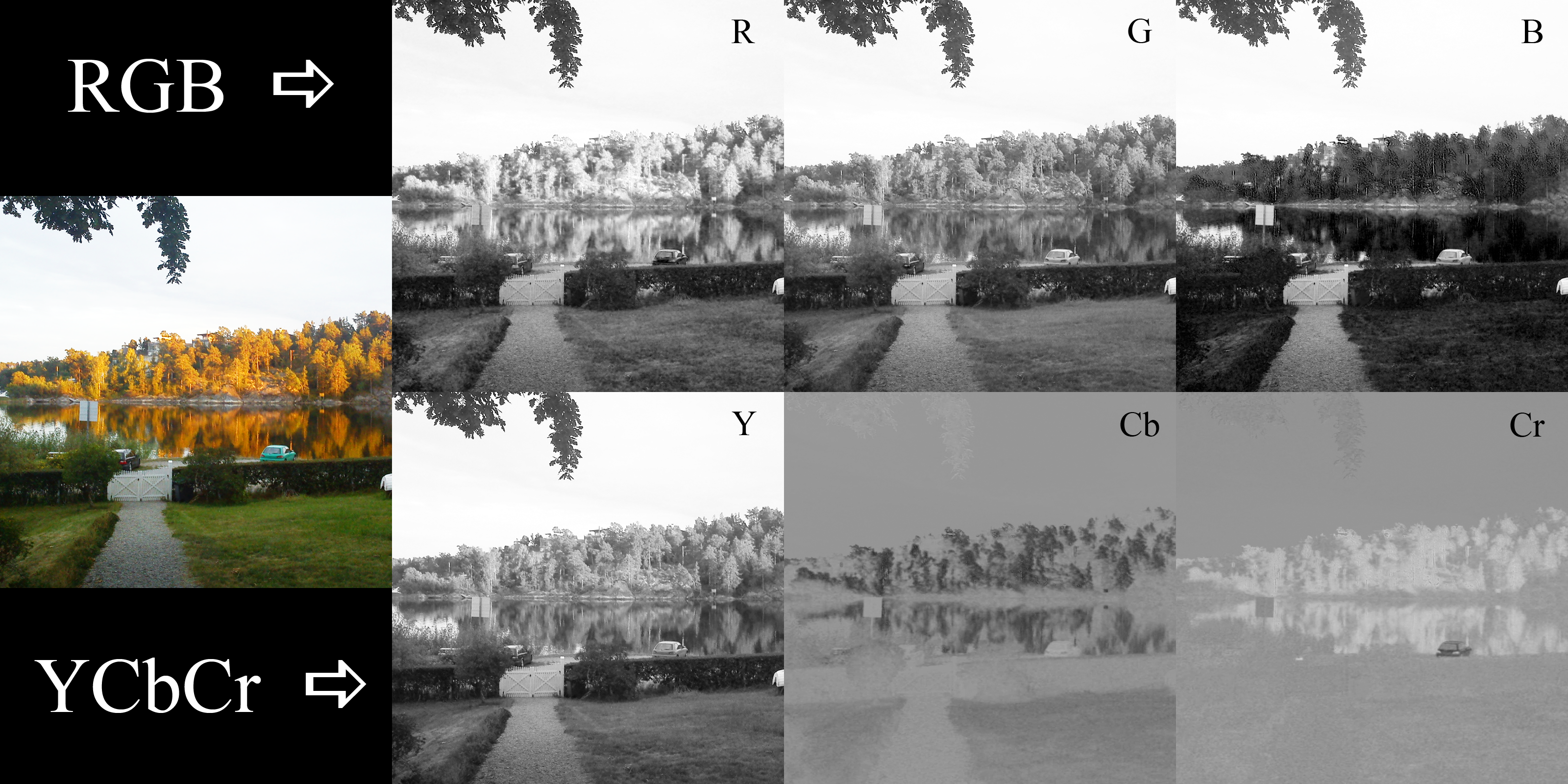
视频帧中的每个像素通过点亮三个子像素显示在计算机屏幕上,分别对应红、绿、蓝三色。在 图 5.5 的顶行中,这些 颜色分量在右侧分别独立展示。 可以看出,这些颜色通道(RGB)彼此相当相似, 这是因为三者都受亮度,即每个像素的整体明暗程度的影响。重复存储同一信息三次是低效的,因此 H.264 等视频编码方案并不将像素存储为 $(R, G, B)$,而是存储 $(Y, Cb, Cr)$,其中
如 图 5.5 底行所示,
$Y$、$Cb$ 和 $Cr$ 通道现在彼此不那么相似了。后两个通道也显得更为“褪色”,而事实证明,这意味着可以用更少的比特来表示图像。此外,人类视觉系统对亮度(大致为 $Y$)误差的敏感度远高于
另外两个通道。这也被加以利用:以较低精度表示色度通道,从而进一步减少比特数。
解压缩时,我们需要从 $(Y, Cb, Cr)$ 恢复为 $(R, G, B)$ 以便在屏幕上显示像素。假设我们 已算出某个像素在 $(Y, Cb, Cr)$ 空间中的颜色为 $Y=180$、$Cb=80$ 和 $Cr=150$。这对应什么 $(R, G, B)$ 颜色? 答案是将 $Y$、$Cb$ 和 $Cr$ 的值代入上述方程并求解 所得的线性方程组,即
视频帧中的每个像素通过点亮三个子像素显示在计算机屏幕上,分别对应红、绿、蓝三色。在 图 5.5 的顶行中,这些 颜色分量在右侧分别独立展示。 可以看出,这些颜色通道(RGB)彼此相当相似, 这是因为三者都受亮度,即每个像素的整体明暗程度的影响。重复存储同一信息三次是低效的,因此 H.264 等视频编码方案并不将像素存储为 $(R, G, B)$,而是存储 $(Y, Cb, Cr)$,其中
| \begin{equation} \begin{cases} \begin{array}{rrrl} Y = & \bs 0.299 & \bs R + 0.587 & \bs G + 0.114 & \bs B,\\ Cb = & \bs -0.169 & \bs R - 0.331 & \bs G + 0.500 & \bs B + 128,\\ Cr = & \bs 0.500 & \bs R - 0.419 & \bs G - 0.081 & \bs B + 128. \end{array} \end{cases} \end{equation} | (5.4) |
解压缩时,我们需要从 $(Y, Cb, Cr)$ 恢复为 $(R, G, B)$ 以便在屏幕上显示像素。假设我们 已算出某个像素在 $(Y, Cb, Cr)$ 空间中的颜色为 $Y=180$、$Cb=80$ 和 $Cr=150$。这对应什么 $(R, G, B)$ 颜色? 答案是将 $Y$、$Cb$ 和 $Cr$ 的值代入上述方程并求解 所得的线性方程组,即
| \begin{equation} \begin{cases} \begin{array}{rrrl} 0.299 &\bs R + 0.587 &\bs G + 0.114 &\bs B = &\bs 180,\\ -0.169 &\bs R - 0.331 &\bs G + 0.500 &\bs B = &\bs -48,\\ 0.500 &\bs R - 0.419 &\bs G - 0.081 &\bs B = &\bs 22. \end{array} \end{cases} \end{equation} | (5.5) |
例 5.2:
电子电路
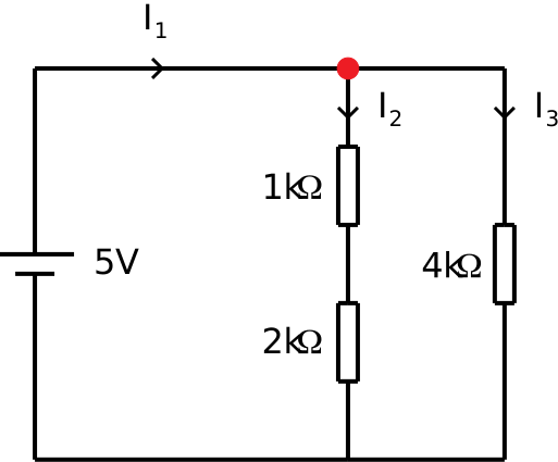
对于下面的电子电路,我们希望计算 电流 $I_1$、$I_2$ 和 $I_3$。 Kirchoff 电压定律指出,沿电路中的闭合回路行进时,各电压之和等于 零。若将其应用于电路的左半部分,我们得到 $5V - I_2 1\mathrm{k}\Omega - I_2 2\mathrm{k}\Omega = 0$。若将其应用于电路的外回路,我们得到 $5V - I_3 4\mathrm{k}\Omega = 0$。最后, 可在电路中的红点处运用 Kirchoff 电流定律 得到第三个方程 $I_1 = I_2 + I_3$。总之,这 给出如下方程组
其中已去掉单位。由此可解出
$I_1$、$I_2$ 和 $I_3$。求解这类方程组是本章其余部分的
主题。
对于下面的电子电路,我们希望计算 电流 $I_1$、$I_2$ 和 $I_3$。 Kirchoff 电压定律指出,沿电路中的闭合回路行进时,各电压之和等于 零。若将其应用于电路的左半部分,我们得到 $5V - I_2 1\mathrm{k}\Omega - I_2 2\mathrm{k}\Omega = 0$。若将其应用于电路的外回路,我们得到 $5V - I_3 4\mathrm{k}\Omega = 0$。最后, 可在电路中的红点处运用 Kirchoff 电流定律 得到第三个方程 $I_1 = I_2 + I_3$。总之,这 给出如下方程组
| \begin{equation} \begin{cases} 1000 I_2 + 2000 I_2 \hid{+ 4000 I_3} = 5,\\ \hid{1000 I_1 + 2000 I_2 +} 4000 I_3 = 5,\\ \hid{1000}I_1\hid{2000} -I_2\hid{4000}-I_3 = 0,\\ \end{cases} \end{equation} | (5.6) |
例 5.3:
用三个点拟合圆
有些问题虽然非线性,但在换元之后可以转化为线性方程组。这里我们用三个点拟合圆的问题来说明这一点。 圆由其圆心 $(u,v)$ 和半径 $r$ 确定。点 $(x_1,y_1)$ 在该圆上 当且仅当
由于有 $3$ 个未知数($u$、$v$ 和 $r$),人们可能会预期需要 $3$ 个方程。
因此,也许需要三个点($(x_1,y_1)$、$(x_2,y_2)$ 和 $(x_3,y_3)$)来确定一个圆。
过三个点 $(-2,3)$、$(-1,1)$ 和 $(-1,2)$ 的圆是什么?
这给出由 3 个非线性方程组成的方程组
将方程中的平方项展开,我们得到
整理各项后,我们有
引入 $w = r^2-u^2-v^2$ 后,我们得到一个线性方程组
再次注意,这个看似非线性的问题可以转化为线性方程组。
求解之后,我们得到 $w$、$u$ 和 $v$ 的值,随后可利用 $w = r^2-u^2-v^2$,即 $r^2 = w+u^2+v^2$,求出半径。
上述例子见 交互图 5.7。
有些问题虽然非线性,但在换元之后可以转化为线性方程组。这里我们用三个点拟合圆的问题来说明这一点。 圆由其圆心 $(u,v)$ 和半径 $r$ 确定。点 $(x_1,y_1)$ 在该圆上 当且仅当
| \begin{equation} (x_1-u)^2 + (y_1-v)^2 = r^2 . \end{equation} | (5.7) |
| \begin{equation} \begin{cases} (-2-u)^2 + (3-v)^2 = r^2 ,\\ (-1-u)^2 + (1-v)^2 = r^2 ,\\ (-1-u)^2 + (2-v)^2 = r^2 .\\ \end{cases} \end{equation} | (5.8) |
| \begin{equation} \begin{cases} 4+4u+u^2 + 9-6v+v^2 = r^2 ,\\ 1+2u+u^2 + 1-2v+v^2 = r^2 ,\\ 1+2u+u^2 + 4-4v+v^2 = r^2 .\\ \end{cases} \end{equation} | (5.9) |
| \begin{equation} \begin{cases} (r^2 - u^2 - v^2) -4u +6v = 13 ,\\ (r^2 - u^2 - v^2) -2u +2v = 2 ,\\ (r^2 - u^2 - v^2) -2u +4v = 5 .\\ \end{cases} \end{equation} | (5.10) |
| \begin{equation} \begin{cases} w -4u +6v = 13 ,\\ w -2u +2v = 2 ,\\ w -2u +4v = 5 .\\ \end{cases} \end{equation} | (5.11) |
上述例子见 交互图 5.7。
例 5.4:
4000 年前的巴比伦问题
巴比伦泥板上就记载着线性方程组。其中一个问题如下:
“有两块田地,总面积为 1800 平方码。一块每平方码产粮 2/3 蒲式耳,另一块每平方码产粮 1/2 蒲式耳。若总产量为 1100 蒲式耳,每块田地的面积是多少?”
为每块田地的面积引入一个变量,即第一块 $x_1$ 平方码,第二块 $x_2$ 平方码。则该问题可改写为
由此可解出 $x_1$、$x_2$。
求解这类方程组是本章其余部分的主题。
巴比伦泥板上就记载着线性方程组。其中一个问题如下:
“有两块田地,总面积为 1800 平方码。一块每平方码产粮 2/3 蒲式耳,另一块每平方码产粮 1/2 蒲式耳。若总产量为 1100 蒲式耳,每块田地的面积是多少?”
为每块田地的面积引入一个变量,即第一块 $x_1$ 平方码,第二块 $x_2$ 平方码。则该问题可改写为
| \begin{equation} \begin{cases} \begin{array}{rrrl} \frac{2}{3} x_1 & \bfm + & \bfm \frac{1}{2} x_2 & \bfm = 1100, \\ x_1 & \bfm + & \bfm x_2 & \bfm = 1800. \\ \end{array} \end{cases} \end{equation} | (5.12) |
求解方程组有许多可能的方法,你 很可能以前已经学过其中一些。然而,高斯 消元法提供的是一种始终有效的方法。你可以 把它想象成一本食谱:只要按步骤操作,就总能得到同样的 美味佳肴。在我们的情形下,最终结果虽不可食用,但会得到一个具有 三角形结构的方程组,因此称为三角方程组。 这一点可见于 图 5.8。
$\begin{array}{rrrl} 6 & \!\!\!\!\!\! x + &\!\!\!\!\!\!\!y - 4 &\!\!\!\!\!\!z = \hid{-}4 \\ & 2 &\!\!\!\!\!\!y + 3 &\!\!\!\!\!\!z = -5 \\ & & 11 &\!\!\!\!\!\!z = -33 \\ \end{array}$
高斯消元法的目标是从任意线性方程组 出发,将其变换为三角方程组。这 只需运用三条简单规则,如下述 定理所示。
定理 5.1:
高斯消元法则
若我们执行下列操作,线性方程组的解保持不变:
此处,我们将该定理的证明推迟到 5.7.1 节,
届时为完整起见也会再次陈述这一定理。
若我们执行下列操作,线性方程组的解保持不变:
- 交换两行的顺序,
- 将某一行乘以一个常数 $\neq 0$,或
- 将另一行的倍数加到某一行上。
作为一个例子,假设我们有如下方程组,
| \begin{equation} \begin{cases} \begin{array}{rl} -x + \hid{4} y =& \!\!\!\! 8,\\ 2 x + 4y =& \!\!\!\!-10. \end{array} \end{cases} \end{equation} | (5.13) |
| \begin{equation} \begin{cases} -x + \hid{6} y = 8,\\ \hid{-x+}6y = 6, \end{cases} \end{equation} | (5.14) |
上面的例子易于求解,因为我们能使用 整数倍数。一般而言,这并不总能做到。例如考虑
| \begin{equation} \begin{cases} 2 x + 3 y = -5, \\ 5 x + 2 y = 4. \end{cases} \end{equation} | (5.15) |
交互图 5.9:
我们从处理最下方的方程开始。现在要消去第一个变量,此处为 $\hid{x}$。
为此,我们在右侧展示一些草稿计算。我们将第一个方程复制到草稿区。
$\Big\{\begin{array}{l} 2 x + 3 y = -5 \\ 5 x + 2 y = 4 \end{array}$
$2 x + 3 y = -5$
$\Big\{\begin{array}{rl} \class{hidden}{2 x + 3 y} & \class{hidden}{= -5} \\ \class{hidden}{11 y} & \class{hidden}{= -33} \end{array}$
$\class{hidden}{\Big\{}\begin{array}{l} 2 x + 3 y = -5 \\ \class{hidden}{5 x + 2 y = 4} \end{array}$
$2 x + 3 y = -5$
$\Big\{\begin{array}{l} 2 x + 3 y = -5 \\ \textcolor{red}{5} x + 2 y = 4 \end{array}$
$\textcolor{red}{5}\class{hidden}{(2 x + 3 y) = 5 (-5) }$
$\textcolor{red}{5}\class{hidden}{(2 x + 3 y) = 5 (-5) }$
$\class{hidden}{5}(2 x + 3 y) = \class{hidden}{5} (-5)$
$\textcolor{red}{5} (2 x + 3 y) = \textcolor{red}{5} (-5)$
$5 x + 2 y = 4$
$5 x + 2 y = 4$
$\class{hidden}{2}(5 x + 2 y) = \class{hidden}{2}(4)$
$\Big\{\begin{array}{l} \textcolor{#00dd00}{2} x + 3 y = -5 \\ 5 x + 2 y = 4 \end{array}$
$\textcolor{#00dd00}{2}$
$\textcolor{#00dd00}{2}$
$\textcolor{#00dd00}{2}\class{hidden}{(5 x + 2 y) =}\textcolor{#00dd00}{2}\class{hidden}{(4)}$
_____________________
$(\textcolor{red}{5}\cdot 2 - \textcolor{#00dd00}{2}\cdot 5) x + (\textcolor{red}{5} \cdot 3 - \textcolor{#00dd00}{2} \cdot 2) y = (\textcolor{red}{5})(-5) - \textcolor{#00dd00}{2}(4)$
$\Leftrightarrow$
$11 y = -33$
$\class{hidden}{\Big\{}\begin{align*} \class{hidden}{2 x + 3 y} & \class{hidden}{= -5} \\ 11 y & = -33 \end{align*}$
$\class{hidden}{5(2 x + 3 y) = }\textcolor{red}{5}\class{hidden}{(-5)}$
$\class{hidden}{2(5 x + 2 y) =}\textcolor{#00dd00}{2}\class{hidden}{(4)}$
$\class{hidden}{\Big\{}\begin{align*} \class{hidden}{2 x + 3 y} & \class{hidden}{= -5} \\ 11 y & = -33 \end{align*}$
$\class{hidden}{\Big\{}\begin{align*} 2 x + 3 y & = -5 \\ \class{hidden}{11 y} & \class{hidden}{= -33} \end{align*}$
$2 x + 3 y = -5$
$\textcolor{red}{5}\class{hidden}{(2 x + 3 y) = 5 (-5) }$
$\class{hidden}{5(2 x + 3 y) =}\textcolor{red}{5}\class{hidden}{(-5)}$
$5 x + 2 y = 4$
$\textcolor{#00dd00}{2}\class{hidden}{(5 x + 2 y) = 2(4)}$
$\class{hidden}{2(5 x + 2 y) =}\textcolor{#00dd00}{2}\class{hidden}{(4)}$
$\class{hidden}{\Big\{}\begin{align*} \class{hidden}{2 x + 3 y} & \class{hidden}{= -5} \\ 11 y & = -33 \end{align*}$
有时无法在下方的行中消去第一个变量, 因为它不在第一行中。例如
| \begin{equation} \begin{cases} \begin{array}{rrrl} 3 & \bs x_2 - 6 & \bs x_3 = -21, \\ 2 x_1 + 4 & \bs x_2 - 2 & \bs x_3 = \hid{-}16, \\ - x_1 - 7 & \bs x_2 + 2 & \bs x_3 = -27. \\ \end{array} \end{cases} \end{equation} | (5.16) |
| \begin{equation} \begin{cases} \begin{array}{rrrl} 2 & \!\!\!\!\!\! x_1 + 4 &\!\!\!\!\!\!\!x_2 - 2 &\!\!\!\!\!\!x_3 = \hid{-}16, \\ - & \!\!\!\!\!\! x_1 - 7 &\!\!\!\!\!\!x_2 + 2 &\!\!\!\!\!\!x_3 = -27, \\ & 3 &\!\!\!\!\!\!x_2 - 6 &\!\!\!\!\!\!x_3 = -21. \\ \end{array} \end{cases} \end{equation} | (5.17) |
| \begin{equation} \begin{cases} \begin{array}{rrrl}\! 2 x_1 + 4&\!\!\!\!\!\!x_2 - 2&\!\!\!\!\!\!x_3 = \hid{-}16, \\ -10&\!\!\!\!\!\!x_2 + 2&\!\!\!\!\!\!x_3 = -38, \\ 3&\!\!\!\!\!\!x_2 - 6&\!\!\!\!\!\!x_3 = -21. \\ \end{array} \end{cases} \end{equation} | (5.18) |
| \begin{equation} \begin{cases} \begin{array}{rrrl} 2 x_1 + 4 x_2 - 2 x_3 & = 16, \\ -10 x_2 + 2 x_3 & = -38, \\ -54 x_3 & = -324.\\ \end{array} \end{cases} \end{equation} | (5.19) |
到目前为止,我们只遇到过恰有一个解的方程组。情况并非总是如此,如下所示
| \begin{equation} \begin{cases} \begin{array}{rl} 5 &\bs x + 2 y = 4,\\ 10 &\bs x + 4 y = 13. \end{array} \end{cases} \end{equation} | (5.20) |
| \begin{equation} \begin{cases} \begin{array}{rl} 5 x + 2 &\bs y = 4\\ &\bs 0 = 5 \end{array} \end{cases} \end{equation} | (5.21) |
| \begin{equation} \begin{cases} 10 x + 4 y = 8,\\ 10 x + 4 y = 13. \end{cases} \end{equation} | (5.22) |
无解并非唯一的特殊情况。例如,假设 我们有如下方程组,
| \begin{equation} \begin{cases} \begin{array}{rll} - &\bs x + &\bs y = \hid{-}8,\\ 3 &\bs x - 3 &\bs y = -24. \end{array} \end{cases} \end{equation} | (5.23) |
| \begin{equation} \begin{cases} \begin{array}{rl} -x + y & \!\!\!\!= 8,\\ 0 & \!\!\!\!= 0. \end{array} \end{cases} \end{equation} | (5.24) |
| \begin{equation} \begin{cases} \begin{array}{rl} -x + t &\bsfyra = 8,\\ y &\bsfyra = t,\\ \end{array} \end{cases} \end{equation} | (5.25) |
| \begin{equation} \begin{cases} x = -8 + t,\\ y = \class{hidden}{-}0 + t.\\ \end{cases} \end{equation} | (5.26) |
$\textcolor{#009600}{S = \begin{pmatrix} -8\\ 0 \end{pmatrix}}$
$\textcolor{#c80000}{\mathrm{\bf d} = \begin{pmatrix} 1\\ 1 \end{pmatrix}}$
$P(t) = S + \mathrm{\bf d}$
$-x + y = 8$
$3x - 3y = -24$
另一种看法是回到原方程,
| \begin{equation} \begin{cases} \begin{array}{rll} - &\bs x + &\bs y = \hid{-}8,\\ 3 &\bs x - 3 &\bs y = -24. \end{array} \end{cases} \end{equation} | (5.27) |
| \begin{equation} \begin{cases} -x + y = 8,\\ -x + y = 8. \end{cases} \end{equation} | (5.28) |
现在考虑一个含三个方程和三个未知数的方程组,例 如
| \begin{equation} \begin{cases} \begin{array}{rrrl} 2 & \!\!\!\!\!\! x + 4 &\!\!\!\!\!\!\!y - 2 &\!\!\!\!\!\!z = \hid{-}16, \\ - & \!\!\!\!\!\! x - 7 &\!\!\!\!\!\!y + 2 &\!\!\!\!\!\!z = -27, \\ & 3 &\!\!\!\!\!\!y - 6 &\!\!\!\!\!\!z = -21. \\ \end{array} \end{cases} \end{equation} | (5.29) |
在其他情形中,两个方程表示同一平面。这可能 是因为它们系数相同,或一个方程等于 另一个方程乘以常数。此时存在整个平面满足 这两个方程,如 交互图 5.12 第三步中虚线平面所示。整个 方程组的解则是该(二重)平面与第三个平面的交线。这对应整条解直线,如 图中实线黑色直线所示。
方程组有解的最后一种情形是:三个方程都表示同一平面,例如方程组
| \begin{equation} \begin{cases} \begin{array}{rrrl} & \bs x + \!\!\!\!&\bs y + &\bs z = 1,\\ 2&\bs x + 2&\bs y + 2&\bs z = 2,\\ 3&\bs x + 3&\bs y + 3&\bs z = 3.\\ \end{array} \end{cases} \end{equation} | (5.30) |
对于含两个方程和两个未知数的方程组,若要无解, 表示两个方程的两条直线必须平行,如 交互图 5.10 所示。三维 情形并非如此。例如考虑如下 方程组。
| \begin{equation} \begin{cases} \begin{array}{rrrl} 3 \sqrt{6}&\bs x + 3&\bs y + 3&\bs z = \sqrt{6}\\ -3 \sqrt{6}&\bs x + 3&\bs y + 3&\bs z = \sqrt{6}\\ & -6&\bs y - 6&\bs z = \sqrt{6}\\ \end{array} \end{cases} \end{equation} | (5.31) |
| \begin{equation} \begin{cases} \begin{array}{rrrl} 3 \sqrt{6}&\bs x + 3&\bs y + 3&\bs z = \sqrt{6},\\ & 6&\bs y + 6&\bs z = 2\sqrt{6},\\ & -6&\bs y - 6&\bs z = \sqrt{6}.\\ \end{array} \end{cases} \end{equation} | (5.32) |
| \begin{equation} \begin{cases} \begin{array}{rrrl} 3 \sqrt{6}&\bs x + 3&\bs y + 3&\bs z = \sqrt{6},\\ & 6&\bs y + 6&\bs z = 2\sqrt{6},\\ & & &\bs 0 = 3\sqrt{6}.\\ \end{array} \end{cases} \end{equation} | (5.33) |
一种特殊情形是两个方程表示同一平面, 而第三个方程表示另一个与它们平行、但不重合的平面。 该例见 图 5.13 的第三步,其中虚线平面 满足两个方程,另一个平面满足第三个 方程。同样,该方程组无解。
最后一种无解情形是两个 平面彼此平行(且互不相同)。 第三个平面沿两条直线与这两个平行平面相交 (在 交互图 5.13 第 4 步中以虚线标出),但不存在同时属于三个平面的点,因此该方程组 无解。
总之,我们可以看到,一个方程组要么有
- 恰有一个解,
- 无解,或
- 无穷多解。
一种特殊情形是所有方程右端均为零,如下例所示。
| \begin{equation} \begin{cases} \begin{array}{rrrl} 2 x_1 + 5 & \bs x_2 + 3 & \bs x_3 = 0, \\ 4 x_1 + 2 & \bs x_2 +\hid{3}& \bs x_3 = 0, \\ 2 x_1 - 3 & \bs x_2 - 2 & \bs x_3 = 0, \\ \end{array} \end{cases} \end{equation} | (5.34) |
| \begin{equation} \begin{cases} \begin{array}{rrrl} 2 x_1 + 5 & \bs x_2 + 3 & \bs x_3 = 0, \\ 8 & \bs x_2 + 5 & \bs x_3 = 0, \\ 8 & \bs x_2 + 5 & \bs x_3 = 0. \\ \end{array} \end{cases} \end{equation} | (5.35) |
| \begin{equation} \begin{cases} \begin{array}{rrrl} 2 x_1 + 5 & \bs x_2 + 3 & \bs x_3 = 0, \\ 8 & \bs x_2 + 5 & \bs x_3 = 0, \\ & & \bs 0 = 0. \\ \end{array} \end{cases} \end{equation} | (5.36) |
| \begin{equation} \begin{cases} \begin{array}{rrrl} 2 x_1 + 5 & \bs x_2 + 3 & \bs t = 0, \\ 8 & \bs x_2 + 5 & \bs t = 0, \\ & & \bs\bs x_3 = t. \\ \end{array} \end{cases} \end{equation} | (5.37) |
| \begin{equation} \begin{cases} \begin{array}{rrl} x_1 = & \bs \frac{1}{16} & \bs t, \\ x_2 = & \bs -\frac{5}{8} & \bs t, \\ x_3 = & \bs &\bs t, \\ \end{array} \end{cases} \end{equation} | (5.38) |
如我们在 3.6 节 所见,平面 与直线都可以写成隐式和显式两种形式。利用 高斯消元法,可以在两种 形式之间转换。回顾 $P(t_1, t_2) = S + t_1 \vc{d}_1 + t_2 \vc{d}_2$ 所表示的平面 是显式形式,而 $\vc{n}\cdot(P-S)=0$ 是隐式形式的平面。 假设我们有如下平面
| \begin{equation} \begin{cases} x &= \class{hidden}{0 +} \frac{3}{2} t_1, \\ y &= \class{hidden}{0 + \frac{3}{2}} t_1 + t_2, \\ z &= 1 \class{hidden}{\frac{3}{2}}-t_1 + 2 t_2, \end{cases} \end{equation} | (5.39) |
| \begin{equation} \begin{cases} \frac{3}{2} &\bs t_1 \class{hidden}{+2t_2}= x,\\ &\bs t_1 \class{hidden}{2}+ t_2 = y,\\ -&\bs t_1 + 2 t_2 = z - 1.\\ \end{cases} \end{equation} | (5.40) |
| \begin{equation} \begin{cases} &\bs t_1 \class{hidden}{2}+ t_2 = y,\\ -&\bs t_1 + 2 t_2 = z - 1,\\ \frac{3}{2} &\bs t_1 \class{hidden}{+2t_2}= x.\\ \end{cases} \end{equation} | (5.41) |
| \begin{equation} \begin{cases} \begin{array}{rl} t_1 + & \bsfem t_2 = y,\\ 3 & \bsfem t_2 = y + z - 1,\\ \frac{3}{2} & \bsfem t_2 = \frac{3}{2}y - x.\\ \end{array} \end{cases} \end{equation} | (5.42) |
| \begin{equation} \begin{cases} \begin{array}{rl} t_1 \class{hidden}{2}+ t_2 & \bsfem = y,\\ 3 t_2 & \bsfem = y + z - 1,\\ 0 & \bsfem= y + z - 1 - 2(\frac{3}{2}y - x).\\ \end{array} \end{cases} \end{equation} | (5.43) |
| \begin{equation} \begin{cases} \begin{array}{rl} 2x - 2t_1 +t_2 + -1 &\bsfem = 0,\\ y &\bsfem = t_1,\\ z &\bsfem = t_2, \end{array} \end{cases} \end{equation} | (5.44) |
| \begin{equation} \begin{cases} \begin{array}{rlll} x &\bsfem = \frac{1}{2} + t_1 -\frac{1}{2}t_2, \\ y &\bsfem = \class{hidden}{\frac{1}{2} } +t_1, \\ z &\bsfem = \class{hidden}{\frac{1}{2} + t1 \frac{1}{2}} + t_2. \end{array} \end{cases} \end{equation} | (5.45) |
前面各节已给出高斯消元法的示例, 并在可能时给出几何解释。在 下一节中,我们将阐述高斯 消元法为何有效的理论。
5.7.1 高斯消元法则
让我们回到例子 方程组 (5.16),即
| \begin{equation} \begin{cases} \begin{array}{rrrl} 3 & \bs x_2 - 6 & \bs x_3 = -21, \\ 2 x_1 + 4 & \bs x_2 - 2 & \bs x_3 = \hid{-}16, \\ - x_1 - 7 & \bs x_2 + 2 & \bs x_3 = -27. \\ \end{array} \end{cases} \end{equation} | (5.46) |
| \begin{equation} \begin{cases} \begin{array}{rrrrl} 3 \cdot & \bs 5 - 6 \cdot & \bs 6 = & \bstwo 15 - 36 & = -21, \\ 2\cdot 4 + 4 \cdot & \bs 5 - 2 \cdot & \bs 6 = & \bstwo 8 + 20 - 12 & = \hid{-}16, \\ - 4 - 7 \cdot & \bs 5 + 2 \cdot & \bs 6 = & \bstwo -4 -35 + 12 & = -27, \\ \end{array} \end{cases} \end{equation} | (5.47) |
此处引入蕴含 $\Rightarrow$ 与等价 $\Leftrightarrow$ 的概念很有用。 若第一个方程组的每个解 也是第二个方程组的解,我们就说第一个方程组蕴含第二个方程组。若这种关系双向成立,则称两个方程组等价。 因此我们可以写
| \begin{equation} \begin{cases} \begin{array}{rrrrrl} 1 x_1 & \bsfem +& \bsfem 2 x_2 & \bsfem = 1, \\ 2 x_1 & \bsfem +& \bsfem 5 x_2 & \bsfem = 7, \\ \end{array} \end{cases} \Leftrightarrow \begin{cases} \begin{array}{rrrrrl} 1 x_1 & \bsfem +& \bsfem 2 x_2 & \bsfem = 1, \\ & \bsfem +& \bsfem 1 x_2 & \bsfem = 5, \\ \end{array} \end{cases} \end{equation} | (5.48) |
定理 5.2:
高斯消元法则
若我们执行下列操作,线性方程组的解保持不变:
若我们执行下列操作,线性方程组的解保持不变:
- 交换两个方程的顺序,
- 将一个方程乘以常数 $\neq 0$,或
- 将一个方程加上另一方程的倍数。
定理 5.2 中的第一条高斯消元法规则 允许交换两个方程的顺序。不难理解,简单地 重排方程顺序不会改变方程组的 解,即
| \begin{equation} \begin{cases} \begin{array}{rrrl} a_{11} x & \bsfem \, + a_{12} y & \bsfem \, + a_{13} z & \bsfem \, = b_1 , \\ a_{21} x & \bsfem \, + a_{22} y & \bsfem \, + a_{23} z & \bsfem \, = b_2 , \end{array} \end{cases} \Leftrightarrow \begin{cases} \begin{array}{rrrl} a_{21} x & \bsfem \, + a_{22} y & \bsfem \, + a_{23} z & \bsfem \, = b_2 , \\ a_{11} x & \bsfem \, + a_{12} y & \bsfem \, + a_{13} z & \bsfem \, = b_1 . \end{array} \end{cases} \end{equation} | (5.49) |
下一条规则允许我们将一个方程乘以一个不等于 $0$ 的常数。由代数可知,将方程两边 同时乘以非零常数不会改变该方程的解, 因而也不会影响方程组的解。
| \begin{equation} \begin{cases} \begin{array}{rrrll} a_{11} x & \bsfem \, + a_{12} y & \bsfem \, + a_{13} z & \bsfem \, = b_1 , & \bsfem \, \, \, (i) \\ a_{21} x & \bsfem \, + a_{22} y & \bsfem \, + a_{23} z & \bsfem \, = b_2 , & \bsfem \, \, \, (ii) \end{array} \end{cases} \Leftrightarrow \begin{cases} \begin{array}{rrrll} ka_{11} x & \bsfem \, + ka_{12} y & \bsfem \, + ka_{13} z & \bsfem \, = kb_1 , & \bsfem \, \, \, (i') = k (i)\\ a_{21} x & \bsfem \, + a_{22} y & \bsfem \, + a_{23} z & \bsfem \, = b_2 . & \bsfem \, \, \, (ii') = (ii) \end{array} \end{cases} \end{equation} | (5.50) |
另一方面,乘以零会改变 解。例如,$(x,y) = (2, 3)$ 不满足 方程
| \begin{equation} x + y = 1, \, \, \, (i) \end{equation} | (5.51) |
| \begin{equation} 0\cdot (x + y) = 0 \cdot 1. \, \, \, \, (i') = 0 (i) \end{equation} | (5.52) |
第三条规则允许我们将另一行的倍数加到 某一行上。假设解 $(x, y, z)$ 满足方程组
| \begin{equation} \begin{cases} \begin{array}{rrrll} a_{11} x & \bsfem \, + a_{12} y & \bsfem \, + a_{13} z & \bsfem \, = b_1, & \bsfem \, \, \, (i)\\ a_{21} x & \bsfem \, + a_{22} y & \bsfem \, + a_{23} z & \bsfem \, = b_2, & \bsfem \, \, \, (ii)\\ a_{31} x & \bsfem \, + a_{32} y & \bsfem \, + a_{33} z & \bsfem \, = b_3. & \bsfem \, \, \, (iii)\\ \end{array} \end{cases} \end{equation} | (5.53) |
| \begin{equation} \begin{cases} \begin{array}{rrrrll} a_{11} x & \bsfem \, + a_{12} y & \bsfem \, + a_{13} z & \bsfyra = & \bsfem b_1, & \bsfem \, \, \, (i')=(i) \\ (a_{21}+ka_{11}) x & \bsfem \, + (a_{22}+ka_{12}) y & \bsfem \, + (a_{23}+ka_{13}) z & \bsfyra = & \bsfem b_2 + k b_1, & \bsfem \, \, \, (ii') = (ii)+k(i)\\ a_{31} x & \bsfem \, + a_{32} y & \bsfem \, + a_{33} z & \bsfyra = & \bsfem b_3. & \bsfem \, \, \, (iii') = (iii) \\ \end{array} \end{cases} \end{equation} | (5.54) |
$\square$
5.7.2 一般情形
本章已给出线性方程组的示例,它们 要么无解,要么恰有一个解,要么有无穷多 解。本节将讨论一般情形,并严格 证明确实如此。
定理 5.3:
线性方程组的解
线性方程组要么
线性方程组要么
- 无解,或
- 恰有一个解,
- 无穷多解。
一个一般的 线性方程组形如
| \begin{equation} \begin{cases} \begin{array}{rrrrrl} a_{11} x_1 + & \bs a_{12} x_2 + & \bs a_{13} x_3 + & \bs \ldots + & \bs a_{1M} x_M & \bs = b_1,\\ a_{21} x_1 + & \bs a_{22} x_2 + & \bs a_{23} x_3 + & \bs \ldots + & \bs a_{2M} x_M & \bs = b_2,\\ a_{31} x_1 + & \bs a_{32} x_2 + & \bs a_{33} x_3 + & \bs \ldots + & \bs a_{3M} x_M & \bs = b_3,\\ & & & & & \bsfem \vdots\\ a_{N1} x_1 + & \bs a_{N2} x_2 + & \bs a_{N3} x_3 + & \bs \ldots + & \bs a_{NM} x_M & \bs = b_N,\\ \end{array} \end{cases} \end{equation} | (5.55) |
| \begin{equation} \begin{cases} \begin{array}{rl} a_{11} x_1 + & \bs a_{12} x_2 + & \bs a_{13} x_3 + & \bs \ldots & \bsfem + a_{1M} x_M & \bs = b_1,\\ & \bs a'_{22} x_2 + & \bs a'_{13} x_3 + & \bs \ldots & \bsfem + a'_{2M} x_M & \bs = b'_2,\\ & \bs a'_{32} x_2 + & \bs a'_{33} x_3 + & \bs \ldots & \bsfem + a'_{3M} x_M & \bs = b'_3,\\ & & & & & \bsfem \vdots\\ & \bs a'_{N2} x_2 + & \bs a'_{N3} x_3 + & \bs \ldots & \bsfem + a'_{NM} x_M & \bs = b'_N.\\ \end{array} \end{cases} \end{equation} | (5.56) |
现在,同样的程序可应用于带撇常数构成的较小方程组,即 (5.56) 中所有不涉及 $x_1$ 的行。同样有两种情况。要么所有这些方程中,我们要消去的变量 $x_2$ 的系数都为零;要么至少有一个方程中变量 $x_2$ 的系数非零。经重新排序和消元后,要么所有方程中变量 $x_2$ 的系数都为零,要么恰有一个方程中变量 $x_2$ 的系数非零。
这一过程持续进行,直到不再含有未知变量的方程。 最后,可能剩下 $0 = 0$ 型的方程。这些方程可以直接删去。 有三种可能的结果。
第一种情况是若至少有一个 $0 = \hat{b}_{i} \neq 0$ 型的方程, 则方程组无解。一个例子见 方程组 (5.33)。 对于接下来的讨论,我们假设不属于这种情况。
第二种情况是所得方程组呈 三角形,即
| \begin{equation} \begin{cases} \begin{array}{rl} \hat{a}_{11} x_1 + & \bs \hat{a}_{12} x_2 + & \bs \hat{a}_{13} x_3 + & \bs \ldots + & \bsfem \hat{a}_{1M} x_M & \bs = \hat{b}_1,\\ & \bs \hat{a}_{22} x_2 + & \bs \hat{a}_{13} x_3 + & \bs \ldots + & \bsfem \hat{a}_{2M} x_M & \bs = \hat{b}_2,\\ & & \bs \hat{a}_{33} x_3 + & \bs \ldots + & \bsfem \hat{a}_{3M} x_M & \bs = \hat{b}_3,\\ & & & & & \bsfem \vdots\\ & & & & \bsfem \hat{a}_{MM} x_M & \bs = \hat{b}_M,\\ \end{array} \end{cases} \end{equation} | (5.57) |
第三种可能是消元后方程个数少于未知数个数,例如
| \begin{equation} \begin{cases} \begin{array}{rl} \hat{a}_{11} x_1 + & \bs \hat{a}_{12} x_2 + & \bs \hat{a}_{13} x_3 + & \bs \hat{a}_{14} x_4 + & \bsfem \hat{a}_{15} x_M & \bs = \hat{b}_1,\\ & & \bs \hat{a}_{23} x_3 + & \bs \hat{a}_{24} x_4 + & \bsfem \hat{a}_{25} x_5 & \bs = \hat{b}_2,\\ & & & \bs \hat{a}_{34} x_4 + & \bsfem \hat{a}_{35} x_5 & \bs = \hat{b}_3.\\ \end{array} \end{cases} \end{equation} | (5.58) |
| \begin{equation} x_4 = \frac{1}{\hat{a}_{34}}(\hat{b}_3 -\hat{a}_{35} t_{2}) . \\ \end{equation} | (5.59) |
因此,方程组要么无解,要么有唯一解,要么有无穷多解。
$\square$
注意,对于无穷多解的情形,了解解集中有多少自由变量也很有意思。换个说法,就是解集的维数是多少。这由 $\rank$ 的概念来刻画, 将在 第 8 章 中说明。
例 5.5:
系数为零
如上证明中所述,有时在进行 高斯消元法 时,某个变量 在所有剩余方程中的系数都可能变为零。此时 可能只需跳过一步,本例即说明了这一点,
我们将第一方程的 $-2$ 倍加到第二方程,从而在第二 行 中消去 $x_1$;又将第一方程的 $-3$ 倍加到最后一个方程,从而在第三 行 中消去 $x_1$。于是得到
通常消去 $x_1$ 后,下一步会
尝试消去 $x_2$。但本例中
第二个和第三个
行 中 $x_2$ 前的系数都为零。于是我们直接跳过,转而处理下一个变量
$x_3$。这里也是如此,因此我们跳到最后一个变量
$x_4$。消去它后只得到方程 $0=0$,于是可将方程组改写为
由最后一个方程可见 $x_4 = -1$。我们令 $x_2 = s$ 和 $x_3 = t$,再将它们代入上方方程,
由此可得
综上所述,我们有
如上证明中所述,有时在进行 高斯消元法 时,某个变量 在所有剩余方程中的系数都可能变为零。此时 可能只需跳过一步,本例即说明了这一点,
| \begin{equation} \begin{cases} \begin{array}{rrrrrrrl} x_1 & \bfm + & \bfm x_2 & \bfm + & \bfm 2 x_3 & \bfm + & \bfm 3 x_4 & \bfm = 1, \\ 2 x_1 & \bfm + & \bfm 2 x_2 & \bfm + & \bfm 4 x_3 & \bfm + & \bfm 7 x_4 & \bfm = 1, \\ 3 x_1 & \bfm + & \bfm 3 x_2 & \bfm + & \bfm 6 x_3 & \bfm + & \bfm 10 x_4 & \bfm = 2. \\ \end{array} \end{cases} \end{equation} | (5.60) |
| \begin{equation} \begin{cases} \begin{array}{rrrrrrrl} x_1 & \bfm + & \bfm x_2 & \bfm + & \bfm 2 x_3 & \bfm + & \bfm 3 x_4 & \bfm = 1, \\ & & & & & \bfm & \bfm x_4 & \bfm = -1, \\ & & & & & \bfm & \bfm x_4 & \bfm = -1. \\ \end{array} \end{cases} \end{equation} | (5.61) |
| \begin{equation} \begin{cases} \begin{array}{rrrrrrrl} x_1 & \bfm + & \bfm x_2 & \bfm + & \bfm 2 x_3 & \bfm + & \bfm 3 x_4 & \bfm = 1, \\ & & & & & \bfm & \bfm x_4 & \bfm = -1. \\ \end{array} \end{cases} \end{equation} | (5.62) |
| \begin{equation} x_1 + s + 2t + 3(-1) = 1, \end{equation} | (5.63) |
| \begin{equation} x_1 = -s - 2t + 4. \end{equation} | (5.64) |
| \begin{equation} \begin{cases} \begin{array}{rllll} x_1 =& \bstre - & \bs s -2 \bs & t \bs & +4,\\ x_2 =& \bstre & \bs s, \bs & \bs & \\ x_3 =& \bstre & \bs \bs & t, \bs & \\ x_4 =& \bstre & \bs \bs & \bs & -1.\\ \end{array} \end{cases} \end{equation} | (5.65) |
本节我们将介绍 线性相关 和 线性无关,它们是 线性 代数中两个重要概念。不过,我们先从 线性组合 开始,这是另一个也时常用到的概念。定义如下。
定义 5.1:
线性组合
向量 $\vc{u}$ 是向量 $\vc{v}_1,\dots,\vc{v}_n$ 的 线性组合,当 $\vc{u}$ 可表示为
其中 $k_1, k_2, \dots, k_n$ 为标量值。
对于 列向量 记法
(定义 2.5),例如我们曾经看到
$\vc{w}= w_x \vc{e}_1+w_y \vc{e}_2+w_z \vc{e}_3$。也就是说,
三维向量 $\vc{w}$ 是
基 向量 $\vc{e}_1$、$\vc{e}_2$ 和 $\vc{e}_3$ 的 线性组合,标量值分别为 $w_x$、$w_y$ 和 $w_z$。
向量 $\vc{u}$ 是向量 $\vc{v}_1,\dots,\vc{v}_n$ 的 线性组合,当 $\vc{u}$ 可表示为
| \begin{equation} \vc{u} = k_1\vc{v}_1 + k_2\vc{v}_2 + \dots + k_n \vc{v}_n = \sum_{i=1}^{n} k_i \vc{v}_i, \end{equation} | (5.66) |
利用 线性组合 的定义,我们现在来考察 线性相关 和 线性无关 的向量组。
定义 5.2:
线性无关与线性相关
向量组 $\vc{v}_1,\dots,\vc{v}_n$ 称为 线性无关,若方程
仅 有唯一解
若存在至少一个其他解,则该向量组 线性相关。
向量组 $\vc{v}_1,\dots,\vc{v}_n$ 称为 线性无关,若方程
| \begin{equation} k_1\vc{v}_1 + k_2 \vc{v}_2 + \dots + k_n \vc{v}_n = \vc{0}, \end{equation} | (5.67) |
| \begin{equation} k_1 = k_2 = \dots = k_n =0. \end{equation} | (5.68) |
例 5.6:
标准基
三维 标准基 由 基 向量
要判断它们是否 线性无关,可针对此情形列出
式 (5.67),
现在,若改用 列向量 记法(定义 2.5),
我们得到
于是得到 $(k_1, k_2, k_3) = (0,0,0)$,这证明 标准基
是 线性无关 的。
三维 标准基 由 基 向量
| \begin{align} \vc{e}_x & = (1,0,0), \\ \vc{e}_y & = (0,1,0), \\ \vc{e}_z & = (0,0,1). \end{align} | (5.69) |
| \begin{equation} k_1\vc{e}_x + k_2\vc{e}_y + k_3\vc{e}_z = \vc{0}. \end{equation} | (5.70) |
| \begin{align} \vc{0} &= k_1\vc{e}_x + k_2\vc{e}_y + k_3\vc{e}_z = k_1 \begin{pmatrix}1\\ 0 \\ 0\end{pmatrix} + k_2 \begin{pmatrix}0\\ 1 \\ 0\end{pmatrix} + k_3 \begin{pmatrix}0\\ 0 \\ 1\end{pmatrix} \\ &= \begin{pmatrix}k_1\\ 0 \\ 0\end{pmatrix} + \begin{pmatrix}0\\ k_2 \\ 0\end{pmatrix} + \begin{pmatrix}0\\ 0 \\ k_3\end{pmatrix} = \begin{pmatrix}k_1\\ k_2 \\ k_3\end{pmatrix}. \end{align} | (5.71) |
定理 5.4:
线性组合与线性相关
向量组 $\vc{v}_1, \vc{v}_2, \dots, \vc{v}_n$ 中的一个向量 $\vc{v}_1, \vc{v}_2, \dots, \vc{v}_n$ 可表示为其余向量的 线性组合,当且仅当 该向量组 线性相关。
向量组 $\vc{v}_1, \vc{v}_2, \dots, \vc{v}_n$ 中的一个向量 $\vc{v}_1, \vc{v}_2, \dots, \vc{v}_n$ 可表示为其余向量的 线性组合,当且仅当 该向量组 线性相关。
由 线性无关 的定义 (定义 5.2) 可知,若向量组 线性相关,则方程
| \begin{equation} k_1\vc{v}_1 + k_2\vc{v}_2 + \dots + k_n \vc{v}_n = \vc{0} \end{equation} | (5.72) |
| \begin{equation} k_1\vc{v}_1 + k_2\vc{v}_2 + \dots + k_{n-1} \vc{v}_{n-1} = - k_n \vc{v}_n, \end{equation} | (5.73) |
| \begin{equation} \vc{v}_n = -\frac{k_1}{k_n}\vc{v}_1 - \dots - \frac{k_{n-1}}{k_n} \vc{v}_{n-1}. \end{equation} | (5.74) |
反向证明更简单。假设其中一个向量可表示为其余向量的 线性组合。重新编号后,设它为向量 $\vc{v}_n$。于是得到
| \begin{equation} \vc{v}_n = a_1\vc{v}_1 + a_2\vc{v}_2 + \dots + a_{n-1} \vc{v}_{n-1}. \end{equation} | (5.75) |
| \begin{equation} 0 = a_1\vc{v}_1 + a_2\vc{v}_2 + \dots + a_{n-1} \vc{v}_{n-1} - 1\vc{v}_n, \end{equation} | (5.76) |
| \begin{equation} k_1\vc{v}_1 + k_2\vc{v}_2 + \dots + k_{n-1} \vc{v}_{n-1} - k_n\vc{v}_n = 0 \end{equation} | (5.77) |
$\square$
例 5.7:
两个向量 $\vc{u} = (1, 2, 3)$ 和 $\vc{v} = (2, 4, 6)$ 是 线性相关 的。这是因为 $\vc{v}$ 可据 $\vc{v} = 2\vc{u}$ 表示为 $\vc{u}$ 的 线性组合。
两个向量 $\vc{u} = (1, 2, 3)$ 和 $\vc{v} = (2, 4, 6)$ 是 线性相关 的。这是因为 $\vc{v}$ 可据 $\vc{v} = 2\vc{u}$ 表示为 $\vc{u}$ 的 线性组合。
例 5.8:
三个向量 $\vc{u} = (1, 2, 3)$、$\vc{v} = (2, 4, 6)$ 和 $\vc{w} = (1, 0, 7)$ 是 线性相关 的。这是因为 $\vc{v}$ 可据 $\vc{v} = 2\vc{u} + 0\vc{w}$ 表示为 $\vc{u}$ 和 $\vc{w}$ 的 线性组合。由此可以得出结论:向已经 线性相关 的向量组中添加向量,永远不可能使新向量组变为 线性无关。
三个向量 $\vc{u} = (1, 2, 3)$、$\vc{v} = (2, 4, 6)$ 和 $\vc{w} = (1, 0, 7)$ 是 线性相关 的。这是因为 $\vc{v}$ 可据 $\vc{v} = 2\vc{u} + 0\vc{w}$ 表示为 $\vc{u}$ 和 $\vc{w}$ 的 线性组合。由此可以得出结论:向已经 线性相关 的向量组中添加向量,永远不可能使新向量组变为 线性无关。
例 5.9:
单个向量 $\vc{v} = (0, 0, 0)$ 是 线性相关 的。这由 定义 5.2 可得,因为 $k_1\vc{v} = \vc{0}$ 对 $k_1$ 的非零值成立,例如 $k_1 = 5$。同理,仅由一个非 零向量 组成的集合是 线性无关 的。
单个向量 $\vc{v} = (0, 0, 0)$ 是 线性相关 的。这由 定义 5.2 可得,因为 $k_1\vc{v} = \vc{0}$ 对 $k_1$ 的非零值成立,例如 $k_1 = 5$。同理,仅由一个非 零向量 组成的集合是 线性无关 的。
例 5.10:
判断三个向量 $\vc{u} = (1, 2, 3)$、$\vc{v} = (2, 3, 4)$、$\vc{w} = (-1, 0, 1)$ 是否 线性无关。
没有明显办法看出这些向量是 线性相关 的。例如,没有向量等于 $(0, 0, 0)$,也没有向量是另一个向量的简单倍数。我们回到定义:这些向量 线性无关,当且仅当
仅有解 $(k_1, k_2, k_3) = (0, 0, 0)$。现在三个分量各自给出一个方程,从而得到方程组
从第二、第三个方程中消去 $k_1$,得到
现在若我们尝试从第三个方程中消去 $k_2$,得到
该方程组是欠定的(underdetermined),有无穷多解。令 $k_3 = t$ 并代入第二个方程得 $k_2 = 2t$,再将这两个值代入第一个方程得
可化简为 $k_1 = -3t$。由于 $t$ 可以非零,这三个向量是 线性相关 的。例如取 $t = 1$,得 $k_1 = -3$、$k_2 = 2$ 和 $k_3 = 1$,代入 式 (5.78) 得
将前两个向量移到右边,可见 $\vc{w} = 3\vc{u} - 2\vc{v}$。
若我们改换最后一个向量为 $\vc{w}' = (-1, 0, 2)$,则得到如下方程组
消去 $k_1$ 得
最后一个方程给出 $k_3 = 0$,代入第二个方程得 $k_2 = 0$,再将这两个值代入最上方方程得 $k_1=0$。于是 $(k_1, k_2, k_3) = (0, 0, 0)$ 是唯一解,向量 $\vc{u}$、$\vc{v}$ 和 $\vc{w}'$ 因此是 线性无关 的。
判断三个向量 $\vc{u} = (1, 2, 3)$、$\vc{v} = (2, 3, 4)$、$\vc{w} = (-1, 0, 1)$ 是否 线性无关。
没有明显办法看出这些向量是 线性相关 的。例如,没有向量等于 $(0, 0, 0)$,也没有向量是另一个向量的简单倍数。我们回到定义:这些向量 线性无关,当且仅当
| \begin{equation} k_1 \begin{pmatrix}1\\ 2 \\ 3\end{pmatrix} + k_2 \begin{pmatrix}2\\ 3 \\ 4\end{pmatrix} + k_3 \begin{pmatrix}-1\\ 0 \\ 1\end{pmatrix} = \begin{pmatrix}0\\ 0 \\ 0\end{pmatrix} \end{equation} | (5.78) |
| \begin{equation} \begin{cases} \begin{array}{rrrl} k_1 \bsfem & + \ 2 k_2 \bsfem & - \ k_3 \bsfem & = 0,\\ 2 k_1 \bsfem & + \ 3 k_2 \bsfem & & = 0,\\ 3 k_1 \bsfem & + \ 4 k_2 \bsfem & + \ k_3 \bsfem & = 0.\\ \end{array} \end{cases} \end{equation} | (5.79) |
| \begin{equation} \begin{cases} \begin{array}{rrrl} k_1 \bsfem & + \ 2 k_2 \bsfem & - \ \hid{2} k_3 \bsfem & = 0,\\ & k_2 \bsfem & - \ 2 k_3 \bsfem & = 0,\\ & 2 k_2 \bsfem & - \ 4 k_3 \bsfem & = 0.\\ \end{array} \end{cases} \end{equation} | (5.80) |
| \begin{equation} \begin{cases} \begin{array}{rrrl} k_1 \bsfem & + \ 2 k_2 \bsfem & - \ \hid{2} k_3 \bsfem & = 0,\\ & k_2 \bsfem & - \ 2 k_3 \bsfem & = 0,\\ & & 0 \bsfem & = 0.\\ \end{array} \end{cases} \end{equation} | (5.81) |
| \begin{equation} k_1 + \ 4 t - \ t = 0, \end{equation} | (5.82) |
| \begin{equation} -3 \begin{pmatrix}1\\ 2 \\ 3\end{pmatrix} +2 \begin{pmatrix}2\\ 3 \\ 4\end{pmatrix} + 1 \begin{pmatrix}-1\\ 0 \\ 1\end{pmatrix} = \begin{pmatrix}0\\ 0 \\ 0\end{pmatrix}, \end{equation} | (5.83) |
若我们改换最后一个向量为 $\vc{w}' = (-1, 0, 2)$,则得到如下方程组
| \begin{equation} \begin{cases} \begin{array}{rrrl} k_1 \bsfem & + \ 2 k_2 \bsfem & - \hid{2}k_3 \bsfem & = 0,\\ 2 k_1 \bsfem & + \ 3 k_2 \bsfem & & = 0,\\ 3 k_1 \bsfem & + \ 4 k_2 \bsfem & + 2k_3 \bsfem & = 0.\\ \end{array} \end{cases} \end{equation} | (5.84) |
| \begin{equation} \begin{cases} \begin{array}{rrrl} k_1 \bsfem & + \ 2 k_2 \bsfem & - \ \hid{2} k_3 \bsfem & = 0,\\ & k_2 \bsfem & - \ 2 k_3 \bsfem & = 0,\\ & 2 k_2 \bsfem & - \ 5 k_3 \bsfem & = 0.\\ \end{array} \end{cases} \end{equation} | (5.85) |
| \begin{equation} \begin{cases} \begin{array}{rrrl} k_1 \bsfem & + \ 2 k_2 \bsfem & - \ \hid{2} k_3 \bsfem & = 0,\\ & k_2 \bsfem & - \ 2 k_3 \bsfem & = 0,\\ & & k_3 \bsfem & = 0.\\ \end{array} \end{cases} \end{equation} | (5.86) |
定理 5.5:
基定理
- 平面 中的两个向量 $\vc{u}$ 和 $\vc{v}$ 构成一个 基,当且仅当它们 线性无关。
- 三维空间中的三个向量 $\vc{u}$、$\vc{v}$ 和 $\vc{w}$ 构成一个 基,当且仅当它们 线性无关。
- 平面 中的三个或更多向量总是 线性相关 的。
- 三维空间中的四个或更多向量总是 线性相关 的。
前两条定理是双向的,因此我们用 $\Rightarrow$ 标记正向证明,用 $\Leftarrow$ 标记反向证明。
1 $\Rightarrow$:假设 $\vc{u}$ 和 $\vc{v}$ 线性无关。定理 5.4 给出 $\vc{u}$ 不能表示为 $\vc{v}$ 的 线性组合,即 $\vc{u} \neq \lambda \vc{v}$,同理 $\vc{v} \neq \lambda \vc{u}$。这意味着 $\vc{u}$ 和 $\vc{v}$ 不平行,于是由 定理 2.4 可知它们在 平面 中构成一个 基。
1 $\Leftarrow$:假设 $\vc{u}$ 和 $\vc{v}$ 在 平面 中构成一个 基。我们现在证明这意味着 $\vc{u}$ 和 $\vc{v}$ 线性无关。假设它们并非 线性无关,却仍构成一个 基,即表达式 $x_u \vc{u} + x_v \vc{v}$ 可以到达 平面 中的每一点。由于它们 线性相关,定理 5.4 指出我们可以写出 $\vc{u} = \lambda \vc{v}$ 或 $\vc{v} = \lambda\vc{u}$。进一步假设我们可以将 $\vc{u}$ 写为 $\vc{u} = \lambda \vc{v}$(这总可以通过交换 $\vc{u}$ 和 $\vc{v}$ 的标签来实现)。假设我们要用 $\vc{w} = x_u \vc{u} + x_v \vc{v}$ 在这个 基 下描述新向量 $\vc{w}$。这等于 $\vc{w} = x_u \lambda \vc{v} + x_v \vc{v} = (x_u \lambda + x_v) \vc{v} = \mu \vc{v}$,其中 $\mu$ 是等于 $(x_u \lambda + x_v)$ 的标量。这意味着只有与 $\vc{v}$ 平行的向量 $\vc{w}$ 才能用 $x_u \vc{u} + x_v \vc{v}$ 来描述,因此 $\vc{u}$、$\vc{v}$ 不能成为整个平面的 基。
2 $\Rightarrow$:定理 2.5 指出,若不存在同时平行于 $\vc{u}$、$\vc{v}$ 和 $\vc{w}$ 的 平面,则这三个向量在空间中构成一个 基。 假设存在一个与三个向量都平行的 平面 $\pi$。由于它与 $\vc{u}$ 和 $\vc{v}$ 平行,它可以写为
| \begin{equation} \pi: \vc{p} + s\vc{u} + t\vc{v}, \end{equation} | (5.87) |
| \begin{equation} \vc{q} = \vc{p} + s_1\vc{u} + t_1\vc{v}, \end{equation} | (5.88) |
| \begin{equation} \vc{q} + \vc{w} = \vc{p} + s_2\vc{u} + t_2\vc{v}. \end{equation} | (5.89) |
| \begin{equation} \vc{w} = (s_2-s_1)\vc{u} + (t_2-t_1)\vc{v}. \end{equation} | (5.90) |
2 $\Leftarrow$:假设 $\vc{u}$、$\vc{v}$ 和 $\vc{w}$ 在空间中构成一个 基。我们现在证明这意味着 $\vc{u}$、$\vc{v}$ 和 $\vc{w}$ 线性无关。假设它们并非 线性无关,却仍构成一个 基,即表达式 $x_u \vc{u} + x_v \vc{v} + x_w \vc{w}$ 可以到达空间中的每一点。由于它们 线性相关,定理 5.4 指出我们至少可以将其中一个向量写为另两个向量的 线性组合。设其中一个为 $\vc{u}$(否则重新命名向量),我们现在可以将 $\vc{u}$ 写为 $\vc{u} = \lambda_v \vc{v} + \lambda_w \vc{w}$。现在我们要用 $\vc{q} = x_u \vc{u} + x_v \vc{v} + x_w \vc{w}$ 在这个 基 下描述 $\vc{q}$。代入 $\vc{u}$ 的 线性 表达式得 $\vc{q} = x_u (\lambda_v \vc{v} + \lambda_w \vc{w}) + x_v \vc{v} + x_w \vc{w} = (x_u \lambda + x_v) \vc{v} + (x_u \lambda_w + x_w) \vc{w} = \mu_v \vc{v} + \mu_w \vc{w}$,其中 $\mu_v$ 和 $\mu_w$ 是标量。这意味着只有与 $\vc{v}$ 和 $\vc{w}$ 所张成的 平面 平行的向量 $\vc{q}$ 才能用 $x_u \vc{u} + x_v \vc{v} + x_w \vc{w}$ 来描述,因此 $\vc{u}$、$\vc{v}, \vc{w}$ 不能成为整个三维空间的 基。 因此,它们 线性无关。
3:假设 $\vc{u}$、$\vc{v}$ 和 $\vc{w}$ 是 平面 中的向量。先考察 $\vc{u}$ 和 $\vc{v}$。若它们 线性相关,即平行,则整个向量组 $\vc{u}$、$\vc{v}$、$\vc{w}$ 也 线性相关,证明完毕。然而,若 $\vc{u}$ 和 $\vc{v}$ 线性无关,则据 (1) 它们在 平面 中构成一个 基。这意味着 $\vc{w}$ 可表示为 线性组合
4:第 4 条的证明与第 3 条相同。
| \begin{equation} \vc{w} = \lambda_1 \vc{u} + \lambda_2 \vc{v} \end{equation} | (5.91) |
| \begin{equation} \lambda_1 \vc{u} + \lambda_2 \vc{v} + (-1)\vc{w} = 0 \end{equation} | (5.92) |
$\square$
本节将介绍张成的概念。在讨论一组向量作为 线性组合 能“占据”向量空间的多少时,这一概念很有用。我们从定义开始。
定义 5.3:
张成
$\R^n$ 中的向量组 $\{\vc{v}_1,\dots,\vc{v}_q\}$ 称为张成 $\R^n$,若方程
对于每个向量 $\vc{u}$ 都至少有一个解。
$\R^n$ 中的向量组 $\{\vc{v}_1,\dots,\vc{v}_q\}$ 称为张成 $\R^n$,若方程
| \begin{equation} k_1\vc{v}_1 + k_2 \vc{v}_2 + \dots + k_q \vc{v}_q = \vc{u}, \end{equation} | (5.93) |
例 5.11:
判断三个向量 $\vc{u} = (1, 2, 3)$、$\vc{v} = (2, 3, 4)$ 和 $\vc{w} = (-1, 0, 1)$ 是否张成 $\R^3$。
我们利用定义来检验
对于每个 $\vc{u}= (u_1, u_2, u_3)$ 都至少有一个解。
现在三个分量各自给出一个方程,从而得到方程组
从第二、第三个方程中消去 $k_1$,得到
现在若我们尝试从第三个方程中消去 $k_2$,得到
该方程组并非对每个 $\vc{u} = (u_1, u_2, u_3)$ 都有解。事实上,只有当向量落在 $u_1-2 u_2+u_3 = 0$ 所定义的 平面 中时才有解。因此这三个向量不张成 $\R^3$。
若我们改换最后一个向量为 $\vc{w}' = (-1, 0, 2)$,则得到如下方程组
消去 $k_1$ 得
该方程对所有 $\vc{u} = (u_1, u_2, u_3)$ 都可解。因此这三个向量张成 $\R^3$。
最后一个方程给出 $k_3 = u_1-2 u_2+u_3$,代入第二个方程得 $k_2 = 4u_1-5u_2+2u_3$,再将这两个值代入最上方方程得 $k_1=-6 u_1 + 8 u_2 - 3 u_3$。于是我们得到唯一解
对每个 $\vc{u} = (u_1, u_2, u_3)$ 都成立。
判断三个向量 $\vc{u} = (1, 2, 3)$、$\vc{v} = (2, 3, 4)$ 和 $\vc{w} = (-1, 0, 1)$ 是否张成 $\R^3$。
我们利用定义来检验
| \begin{equation} k_1 \begin{pmatrix}1\\ 2 \\ 3\end{pmatrix} + k_2 \begin{pmatrix}2\\ 3 \\ 4\end{pmatrix} + k_3 \begin{pmatrix}-1\\ 0 \\ 1\end{pmatrix} = \begin{pmatrix}u_1\\ u_2 \\ u_3\end{pmatrix} \end{equation} | (5.94) |
| \begin{equation} \begin{cases} \begin{array}{rrrl} k_1 \bsfem & + \ 2 k_2 \bsfem & - \ k_3 \bsfem & = u_1,\\ 2 k_1 \bsfem & + \ 3 k_2 \bsfem & & = u_2,\\ 3 k_1 \bsfem & + \ 4 k_2 \bsfem & + \ k_3 \bsfem & = u_3.\\ \end{array} \end{cases} \end{equation} | (5.95) |
| \begin{equation} \begin{cases} \begin{array}{rrrl} k_1 \bsfem & + \ 2 k_2 \bsfem & - \ \hid{2} k_3 \bsfem & = u_1,\\ & k_2 \bsfem & - \ 2 k_3 \bsfem & = 2u_1-u_2,\\ & 2 k_2 \bsfem & - \ 4 k_3 \bsfem & = 3 u_1-u_3.\\ \end{array} \end{cases} \end{equation} | (5.96) |
| \begin{equation} \begin{cases} \begin{array}{rrrl} k_1 \bsfem & + \ 2 k_2 \bsfem & - \ \hid{2} k_3 \bsfem & = u_1,\\ & k_2 \bsfem & - \ 2 k_3 \bsfem & = 2 u_1-u_2,\\ & & 0 \bsfem & = u_1-2 u_2+u_3.\\ \end{array} \end{cases} \end{equation} | (5.97) |
若我们改换最后一个向量为 $\vc{w}' = (-1, 0, 2)$,则得到如下方程组
| \begin{equation} \begin{cases} \begin{array}{rrrl} k_1 \bsfem & + \ 2 k_2 \bsfem & - \hid{2}k_3 \bsfem & = u_1,\\ 2 k_1 \bsfem & + \ 3 k_2 \bsfem & & = u_2,\\ 3 k_1 \bsfem & + \ 4 k_2 \bsfem & + 2k_3 \bsfem & = u_3.\\ \end{array} \end{cases} \end{equation} | (5.98) |
| \begin{equation} \begin{cases} \begin{array}{rrrl} k_1 \bsfem & + \ 2 k_2 \bsfem & - \ \hid{2} k_3 \bsfem & = u_1,\\ & k_2 \bsfem & - \ 2 k_3 \bsfem & = 2 u_1-u_2,\\ & 2 k_2 \bsfem & - \ 5 k_3 \bsfem & = 3 u_1-u_3.\\ \end{array} \end{cases} \end{equation} | (5.99) |
| \begin{equation} \begin{cases} \begin{array}{rrrl} k_1 \bsfem & + \ 2 k_2 \bsfem & - \ \hid{2} k_3 \bsfem & = u_1,\\ & k_2 \bsfem & - \ 2 k_3 \bsfem & = 2 u_1-u_2,\\ & & k_3 \bsfem & = u_1-2 u_2+u_3.\\ \end{array} \end{cases} \end{equation} | (5.100) |
| \begin{equation} \begin{cases} \begin{array}{lrrr} k_1 & = -6 u_1 \bsfem & + \ 8 u_2 \bsfem & - \ 3 u_3 & \bsfem\\ k_2 & = 4 u_1 \bsfem & - \ 5 u_2 \bsfem & + \ 2 u_3 & \bsfem\\ k_3 & = \hid{1} u_1 \bsfem & - \ 2 u_2 \bsfem & + \ \hid{1} u_3 & \bsfem\\ \end{array} \end{cases} \end{equation} | (5.101) |
定理 5.6:
基的条件
向量组 $\{\vc{u}_1, \vc{u}_2, \ldots, \vc{u}_k\}$ 是 $\R^n$ 中的 基,当且仅当这些向量 线性无关 且张成 $\R^n$。
向量组 $\{\vc{u}_1, \vc{u}_2, \ldots, \vc{u}_k\}$ 是 $\R^n$ 中的 基,当且仅当这些向量 线性无关 且张成 $\R^n$。
假设向量组 $\vc{u}_1, \vc{u}_2, \ldots, \vc{u}_q$ 是 $\R^n$ 的 基。则据 定义 2.10,对每个 $\vc{u}$,方程 $k_1\vc{v}_1 + k_2 \vc{v}_2 + \dots + k_q \vc{v}_q= \vc{u}$ 都有解,因此据 定义 5.3 这些向量张成 $\R^n$。 要证明这些向量 线性无关,我们注意到方程 $ \sum_{i=1}^q k_i \vc{v}_i = \vc{0}$ 有一个解 $k_1=0, k_2=0, \ldots, k_q=0$。据 基 的定义 (定义 2.10),该解是唯一的。这证明这些向量 线性无关。
为完成反向证明,我们假设向量组 $\vc{u}_1, \vc{u}_2, \ldots, \vc{u}_q$ 张成 $\R^n$ 且 线性无关。我们需要证明 $\sum_{i=1}^q k_i \vc{v}_i = \vc{u}$ 对每个 $\vc{u}$ 都恰有一个解。由于这些向量张成 $\R^n$,对每个 $\vc{u}$ 都至少有一个解。假设有两个解 $(k_1, k_2, \ldots, k_q)$ 和 $(k^\prime_1, k^\prime_2, \ldots, k^\prime_q)$。若我们将方程 $\sum_{i=1}^q k^\prime_i \vc{v}_i = \vc{u}$ 从 $\sum_{i=1}^q k_i \vc{v}_i = \vc{u}$ 中减去,得到 $\sum_{i=1}^q (k_i-k^\prime_i) \vc{v}_i = \vc{0}$。由于这些向量 线性无关(定义 5.2),我们有 $(k_i-k^\prime_i) = 0$,但这给出 $k_i=k^\prime_i$,因此两个解相同。
$\square$
假设我们在 平面 中有一个 基,即两个不平行 基 向量 $\vc{e}_1$ 和 $\vc{e}_2$。 此外,假设我们还有另一对不平行向量 $\hat{\vc{e}}_1, \hat{\vc{e}}_2$,它们也构成一个 基。 正如我们上面所见,这两个向量现在可以用前两个向量表示为
| \begin{gather} \hat{\vc{e}}_1 = x_{11} \vc{e}_1 + x_{21} \vc{e}_2,\\ \hat{\vc{e}}_2 = x_{12} \vc{e}_1 + x_{22} \vc{e}_2. \end{gather} | (5.102) |
| \begin{gather} \vc{u} = u_1 \vc{e}_1 + u_2 \vc{e}_2 .\\ \end{gather} | (5.103) |
| \begin{gather} \vc{u} = \hat{u}_1 \hat{\vc{e}}_1 + \hat{u}_2 \hat{\vc{e}}_2.\\ \end{gather} | (5.104) |
| \begin{gather} \vc{u} = \hat{u}_1 (x_{11} \vc{e}_1 + x_{21} \vc{e}_2) + \hat{u}_2 (x_{12} \vc{e}_1 + x_{22} \vc{e}_2), \end{gather} | (5.105) |
| \begin{gather} \vc{u} = (x_{11} \hat{u}_1 + x_{12} \hat{u}_2 ) \vc{e}_1 + (x_{21}\hat{u}_1 + x_{22}\hat{u}_2 ) \vc{e}_2. \end{gather} | (5.106) |
| \begin{gather} u_1 = x_{11} \hat{u}_1 + x_{12} \hat{u}_2, \\ u_2 = x_{21}\hat{u}_1 + x_{22}\hat{u}_2. \end{gather} | (5.107) |
我们将在 第 6 章 中回到 基 变换,该章讨论矩阵这一主题。
